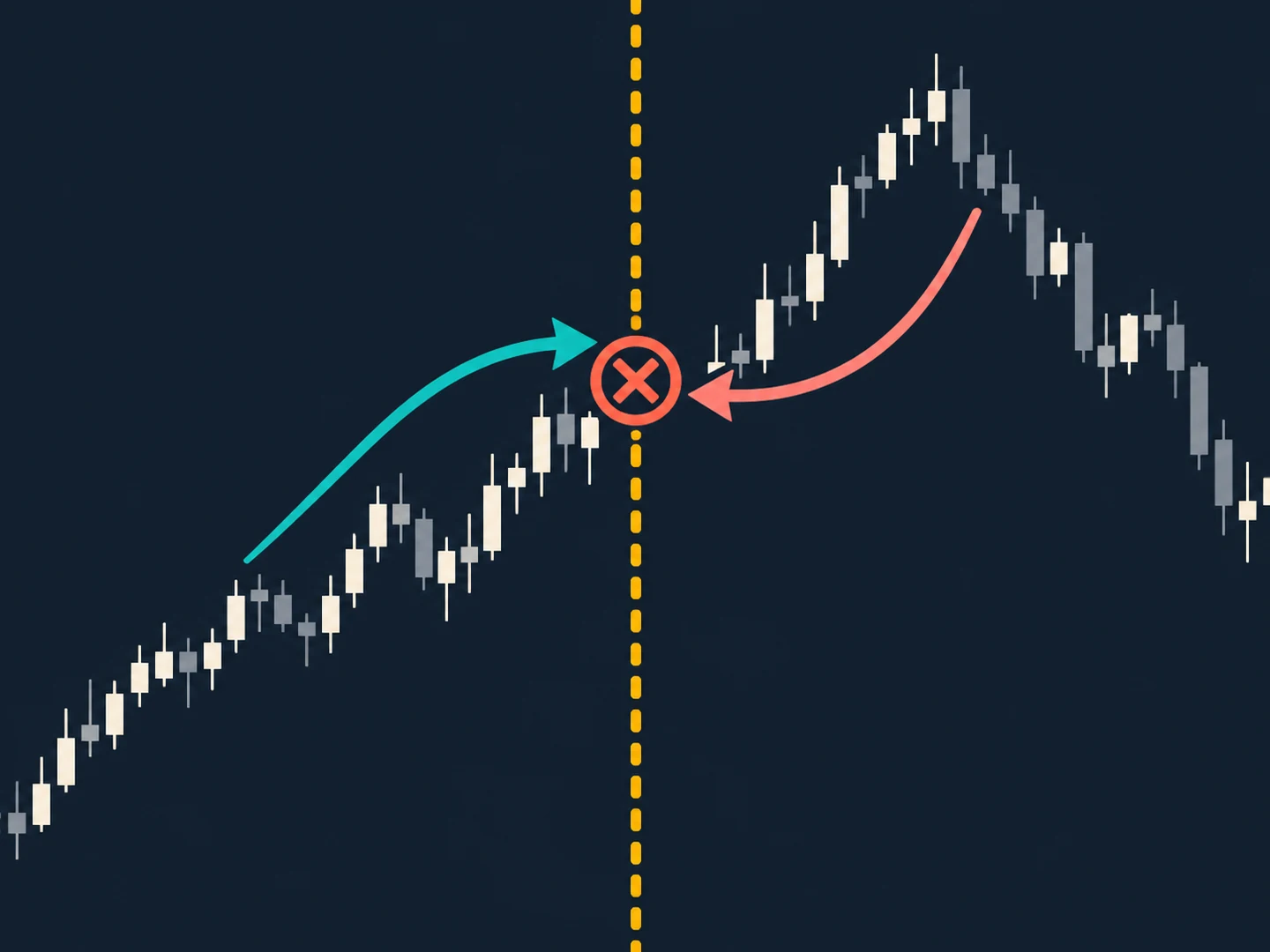
A performance summary often begins with one number: average result per trade. It feels intuitive because it compresses a list into something easy to compare. But the word average is ambiguous, and even a precisely calculated mean can hide a distribution that is highly uneven. A report that calls one statistic typical may lead readers to imagine a representative outcome that the data do not contain.
The arithmetic mean and the median answer different questions. The mean is the sum of observed values divided by the number of observations. The median is the middle value after sorting, or the midpoint of the two central values when the count is even. The mean is sensitive to every observation; the median is less affected by the magnitude of a distant extreme value. Neither is universally better. Their usefulness depends on the question and the shape of the sample.
What does a five-outcome example show about mean and median?
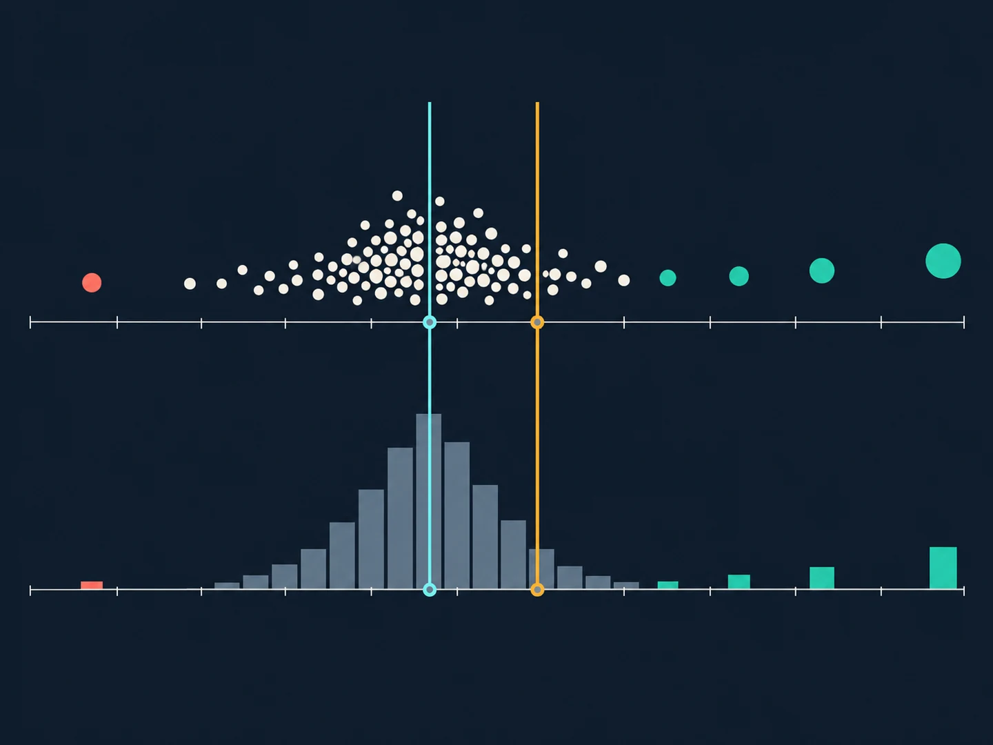
Consider a fictional set of five net outcomes measured in the same unit: minus two, minus one, zero, one, and eleven. The mean is 1.8, while the median is zero. The mean reflects the arithmetic contribution of the large positive observation. The median identifies the center of the ordered list. Neither statement implies that one statistic is a forecast or that a similar result should be expected in another sample.
Now imagine a sample in which most observations cluster near the center and a small number of unusually large outcomes stretch the right tail. The mean may sit well away from most individual results. In a left-skewed sample, a few unusually negative values can pull it in the opposite direction. Reporting the mean without showing spread and shape can make the sample sound more uniform than it is.
Be explicit about what is being averaged
A mean cannot be interpreted until the observation is defined. Is each item one closed trade, one session, one strategy configuration, or one day? Are values gross or net of modeled costs? Are partial exits combined? Are open positions included? Do all observations use the same currency, contract multiplier, and time convention? A mathematically correct calculation over inconsistent units can still be misleading.
Selection matters as much as arithmetic. A sample containing only completed trades excludes periods when no trade occurred. A sample limited to one product, time window, or parameter choice may not represent a broader process. Missing observations, duplicate records, and survivorship or selection filters can change both the mean and median. Document the inclusion rule before interpreting the result.
Report more than a center
A central statistic is only one view of a distribution. Useful context can include the number of observations, a measure of spread, selected quantiles, the range when appropriate, and a visual display such as a histogram or box plot. These summaries reveal whether observations cluster tightly, contain tails, or form multiple groups. They do not remove the need to understand how the sample was formed.
- Sample size and unit: how many observations are included, and what does each one represent?
- Center: report mean and median with unambiguous labels and units.
- Spread: show a defined dispersion measure or quantiles, with method stated.
- Shape: inspect skew, tails, clusters, and unusual values rather than assuming symmetry.
- Net convention: disclose fees, spread, slippage, and any other modeled deductions.
- Coverage: state the date range, inclusion rules, exclusions, and missing-data handling.
Outliers deserve investigation, not automatic deletion. A large observation might be a data error, a legitimate rare event, an aggregation problem, or a feature of the process being studied. Keep a reproducible record of any correction or exclusion and report how conclusions change with and without a disputed point. A robust summary can help describe sensitivity, but it does not make inconvenient observations disappear.
A mean is not expectancy without a model
People sometimes use average trade outcome and expectancy as though they were always interchangeable. In a simple sample, the arithmetic mean is an estimate of the sample's per-observation average under the chosen unit and accounting convention. A broader expectancy claim usually depends on assumptions about how observations are generated, whether the process is stable, how trades are selected, and what costs or constraints apply.
Even a positive historical mean does not establish that a process will continue to have a positive mean. Sampling uncertainty can be large, particularly when the sample is small, observations are dependent, or a few values dominate the sum. If trades overlap or cluster in time, treating each as independent can understate uncertainty. The calculation should match the data-generating and sampling design as closely as the research allows.
Separate frequency from payoff size
A win rate is not an average outcome. It records the proportion of observations classified as wins under a defined sign convention. The sizes of gains and losses add another dimension. Two samples can have the same win rate and different means because the magnitude distribution differs; they can also have similar means but very different medians and tails.
This is why a concise performance table should avoid turning one metric into a full verdict. A high proportion of positive observations does not reveal the size of negative outcomes. A positive mean does not show how often values were near zero, how variable they were, or whether the result depends on a small number of extreme cases. Each statistic describes a different feature.
Compare groups only when their definitions align
Comparing averages across two strategies, periods, or markets can be useful only when the units and sample rules are compatible. One group may contain more observations, a different cost model, a different time horizon, or a different mix of conditions. Normalizing a number does not automatically make the underlying observations comparable.
When groups differ, show the differences rather than hiding them in a single ranking. Report sample counts, date coverage, data-source changes, and relevant design choices. If the comparison was chosen after inspecting many alternatives, explain the search process. A clean table should make caveats easier to see, not bury them beneath decimal precision.
Use a distribution-first review
A practical review begins by defining the observation and inclusion rule. Verify the raw records, calculate center and spread, inspect the shape, and investigate influential observations. Then test whether the main description changes under reasonable alternate windows or groupings. Keep exploratory comparisons separate from a pre-specified confirmation step when possible.
For an educational report, a clear sentence might say that the sample mean was a stated amount after specified modeled costs, the median was another amount, and the distribution was right-skewed with a disclosed number of observations over a stated period. It should then say what the sample cannot establish. This is more informative than calling either statistic the typical result without qualification.
Precision includes the limits
The NIST/SEMATECH handbook describes mean and median as measures of location and discusses how they relate to exploratory data analysis. That framing is useful: a statistic helps summarize a dataset, but interpretation depends on the data's distribution and context. A decimal point does not remove uncertainty, and a familiar summary does not convert a historical sample into a personal financial conclusion.
A careful report uses the mean to describe arithmetic balance and the median to locate the middle, then places both inside a broader account of sample size, spread, shape, coverage, and assumptions. If those details are unavailable, the limitation is itself important information. The objective is not to crown one summary as correct; it is to make clear what each one reveals and what remains unknown.
- Read portfolio risk beyond standalone measures
- Understand sample size and streaks
- Audit historical-test information timing
Sources and further reading
- Measures of LocationNIST/SEMATECH e-Handbook of Statistical Methods