A Win Rate Is an Estimate, Not a Fixed Trait

A win rate is easy to read and easy to overread. Once a report prints “50%,” the number can start to feel like a property of a method, almost like its name or timeframe. It is actually a summary of one defined sample: the number of outcomes labeled wins divided by the number counted. Change the rule for what enters that denominator and the rate can change, even if the underlying decisions do not.

So the percentage needs a question attached to it. Which cases were counted? What qualified as a win? Were the observations comparable? A win rate is an estimate from a record, not a permanent trait and not a forecast. Its usefulness depends on the data and assumptions behind it.

Which event are you counting?

For a simple win rate, each observation is sorted into two groups: win or not win. If 37 of 80 eligible outcomes meet the stated win definition, the sample rate is 37 divided by 80, or 46.25%. That arithmetic is straightforward. The harder part is deciding what an observation is and where the win boundary sits. A completed trade, a position after fees, a decision window, and a full round trip are different units. They should not be mixed without explanation.

The label also needs a rule. Does a win mean a positive result before costs or after costs? Is a scratch trade a third category, or is it grouped with non-wins? How are partial exits combined? None of these definitions is universally correct for every review. What matters is that the rule is written down and applied consistently. Otherwise two people can calculate different rates from the same ledger and both perform the division correctly.

This definition turns a continuous outcome into a binary one. The simplification is useful when the question concerns frequency, but it discards the size of each gain and loss. It also means a small change in classification can move observations across the boundary. A rate without its win rule is missing part of its meaning.

The same percentage can carry different precision

Consider two clearly hypothetical records. One contains 10 wins in 20 observations; another contains 100 wins in 200. Both show a 50% sample win rate. The first fraction is not automatically wrong, and the second is not automatically representative. But under a common, unchanged process with independent observations, the larger sample generally gives a more precise estimate of the same underlying proportion. The percentage alone hides that difference.

A confidence interval can make sampling uncertainty more visible. It gives a range calculated from the observed proportion under a stated method and model. The interval is not a forecast band around future trades. Its width depends on the estimate, the number of observations, and the chosen procedure. A narrow interval can still be misleading if the sample was selected poorly or the model does not fit the records.

A confidence interval describes a procedure

The familiar phrase “95% confidence interval” is often read as “there is a 95% chance the true rate is inside these particular limits.” That is not the usual frequentist interpretation. The confidence level describes the long-run behavior of the interval procedure: if comparable samples were repeatedly drawn under the model and an interval calculated each time, about 95% of those intervals would contain the fixed population proportion. NIST explains confidence intervals in this repeated-sampling way.

For a win rate, the parameter in that explanation is a proportion associated with a defined population or process. The interval does not assign a probability to the next trade being a win, guarantee that a future block of outcomes will fall inside its limits, or say that the process will remain unchanged. Those are different questions and require assumptions the interval alone does not supply.

There is more than one way to calculate an interval for a proportion. Methods can behave differently, especially when the sample is small or the observed rate is near zero or one. NIST describes Wilson and exact binomial approaches and notes that a simple normal approximation may not be accurate enough for some small-sample cases. A report should name the method rather than display unexplained bounds from a default spreadsheet cell.

The binomial model is a useful simplification

A common starting point treats each observation as one of two outcomes and assumes the chance of a win is the same from trial to trial. That is the basic binomial setup described by NIST. Under that model, the observed proportion estimates a fixed success probability. The model is useful because it turns a count and a denominator into a clear statistical question.

Trading records may not behave like repeated draws from one unchanged process. Outcomes can cluster in time, share the same underlying conditions, or come from different rule versions and market settings. If observations are dependent, counting every row as an independent trial can make the evidence look stronger than it is. If the chance of a win changes across groups, one pooled proportion can blur meaningful differences rather than estimate one stable rate.

A larger file does not solve those design problems by itself. Two hundred consecutive observations from one narrow setting may answer a narrower question than a smaller but deliberately defined sample across several settings. The sample size tells how many records were counted. It does not tell whether the records represent the question a reader thinks the rate answers.

The denominator determines the question

A win rate calculated over completed trades answers a question about the outcomes of those completed trades. It does not automatically describe every opportunity, every decision, or every session. If a review includes only trades that were taken, its denominator leaves out moments when no trade occurred. That may be exactly the intended measure, but it should not be mistaken for a rate over all eligible decisions.

Selection rules can change the result too. Excluding incomplete records, omitting a difficult period, or grouping only the cases that fit a later definition changes the sample being summarized. Keep the inclusion rule visible, including missing observations and any filters. A journal that records no-trade sessions can help distinguish “no qualifying decision occurred” from “the record is absent”; see the related guide on what to record when no trade occurred.

Win rate leaves payoff size out

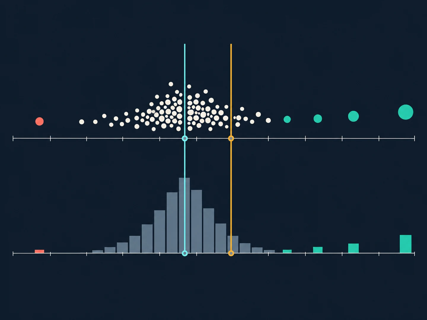
A win rate says how often observations crossed a chosen boundary. It says nothing about how far they crossed it. Two hypothetical samples can each contain the same share of wins while one has small positive outcomes and large negative ones, and the other has a different payoff mix. The sign count alone cannot distinguish them. Mean, median, dispersion, and drawdown answer separate questions; our guide to average versus median trade outcomes explains why a single center statistic also needs context.

For that reason, a win rate should not be treated as a standalone score or goal. A higher sample rate does not, on its own, establish better performance, a more reliable process, or a favorable future result. It is one description of one feature in a defined set of observations.

Report the estimate with its boundaries

A useful report gives the reader enough detail to reconstruct the claim. Before interpreting the percentage, record:

• The observation unit and the exact rule for labeling a win, including how costs, scratches, partial exits, and open outcomes are handled.
• The count of wins and the total denominator alongside the percentage, not the percentage alone.
• The dates, groups, rule versions, exclusions, missing records, and any choice that determined which observations entered the sample.
• The interval method and confidence level, if an interval is reported, plus the assumptions that matter for interpreting it.
• Other measures that answer different questions, such as payoff size or drawdown, kept separate from the win rate rather than blended into one verdict.

A careful sentence might read: “In this hypothetical sample, 100 of 200 included observations met the stated win definition; the reported interval uses a binomial method that assumes a common success probability across trials.” That sentence is less sleek than “the win rate is 50%,” but it keeps the statistic attached to its denominator and model.

The useful question is not whether a win rate looks high or low in isolation. Ask what was counted, why the cases belong together, and which assumptions turn the count into an estimate. A historical or simulated percentage describes its record. It does not promise what a later sample will contain.

• See what average and median trade outcomes reveal
• Read why a short streak can mislead
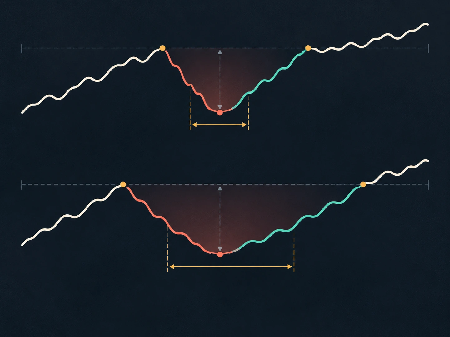
• Compare drawdown depth with duration